02 / Feedback control
Ball-and-plate control
I built a two-axis platform that uses camera feedback to balance a ball. The work covered the mechanism, vision pipeline, dynamics model, and controller implementation.
- My role
- Mechanical build, modeling & software
- Period
- Jan – Apr 2026
- Tools
- Python/OpenCV, Raspberry Pi & MATLAB/Simulink
- Evidence
- Hardware video, simulation model & calculations
The feedback loop
Measure the ball.
Correct the plate.
- 01Camera image
- 02Ball position & estimated velocity
- 03Controller
- 04Plate tilt → servo pulses
Turn an image into a position.
The camera sees pixels; the controller needs a position on the plate. I use a perspective transform to map the camera view into plate coordinates, then convert the detected ball center into a distance from the target.
The vision code filters orange regions and scores their shape to select a ball candidate. An alpha-beta tracker estimates velocity from successive position measurements, so the controller can respond to both position and motion.
One platform, several controllers.
I used the ball-and-plate dynamics to build PID and state-feedback implementations and a discrete LQR design. The saved controller calculations distinguish the hand-tuned runtime gains from a separate model-derived PID version.
PID
Position, velocity, and accumulated error produce a desired acceleration. The model-based version derives gains by matching a desired characteristic polynomial.
State feedback & LQR
The state-space model represents position and velocity on both axes. The LQR solver discretizes that model and computes feedback gains from state and input weights.
MATLAB & Simulink
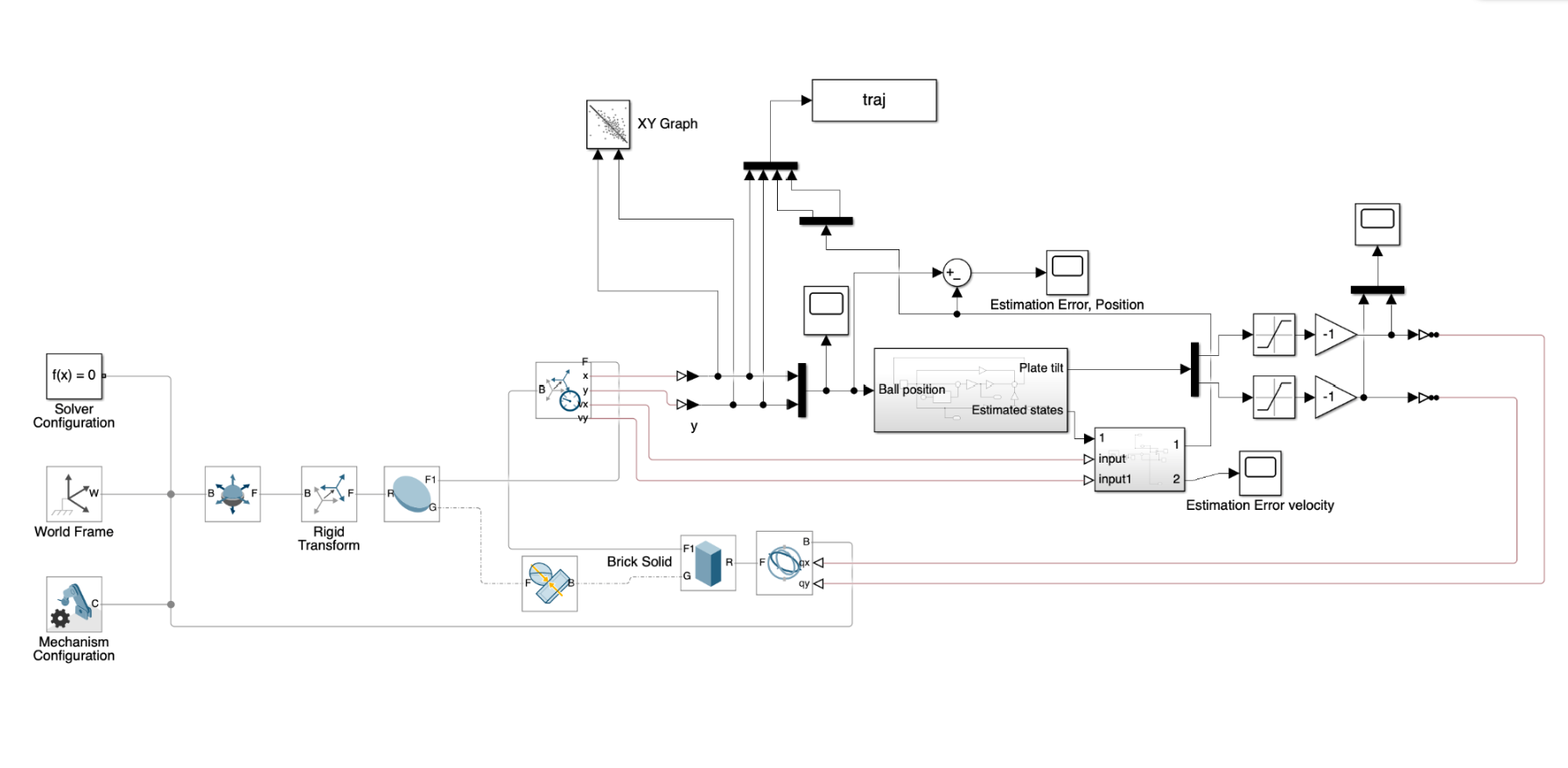
My Simulink model connects the ball-and-plate mechanics with position feedback, state estimation, and plate-tilt commands.
The controller
A requested acceleration becomes a plate-tilt command, then a servo angle and PWM pulse. The software limits plate tilt and the rate at which it changes, keeping commands within the mechanism’s configured range.
Tracking confidence and elapsed time since the last detection determine whether a ball measurement can be used. These checks matter because a camera can lose the ball while the servos still have a command.
Centering and path tracking
I completed the build, modeling, software, and hardware testing, and earned the highest mark in the course.
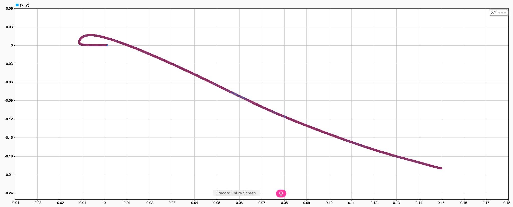
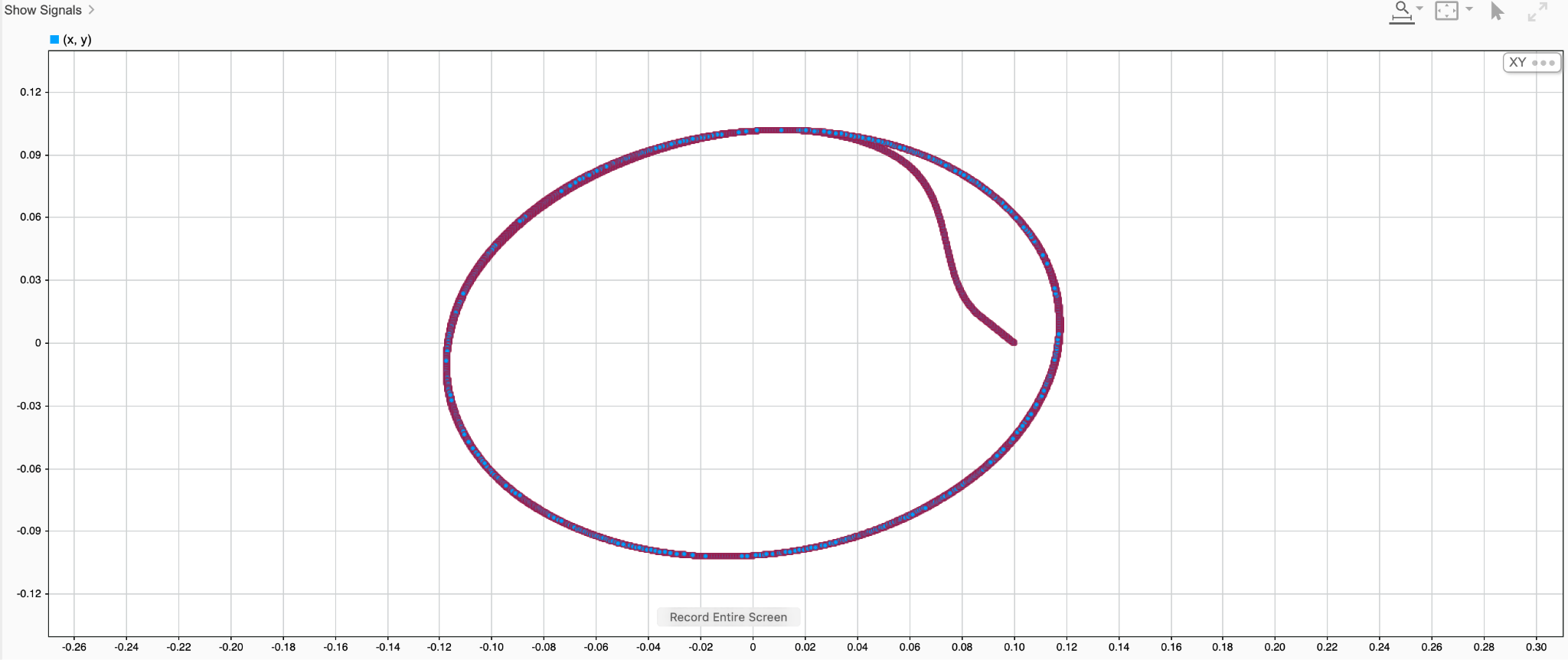
The simulation results cover two cases: returning the ball to the center from an offset starting position and following a circular reference. The X–Y plots below show the path in each case.
Model-derived PID calculations
The saved derivation uses the augmented per-axis state: position error e, error velocity v, and integrated error z.
a = −kpe − kdv − kiz
Matching coefficients of the desired polynomial gives:
kd = 2ζωn + ωi
kp = ωn² + 2ζωnωi
ki = ωn²ωi
With ζ = 1.05, ωn = 2.5 rad/s, and ωi = 0.18 rad/s, the calculated gains are kp = 7.195, kd = 5.430, and ki = 1.125.
Design parameters from the March 2026 calculation document. The final saved runtime uses separate hand-tuned gains; these values are not a measured performance result.